Sinusoidal Alternating Current II
Alternating Current 2
Reactance and Impedance. Series RLC Circuits. Resonance
Summary. By analyzing how the ideal resistor, inductor and capacitor behave under sinusoidal conditions, we introduce the concepts of reactance and impedance. We then study the two-terminal circuits obtained by connecting these components in series, also as a function of frequency. Finally, we look at the phenomenon of series resonance, or voltage resonance.
Before you start.
To get the most out of this lesson, you may find it useful to read the previous module in this series, Alternating Current 1: Sinusoidal Electrical Quantities, which presents some fundamental concepts, including an introduction to the "symbolic method" and to the use of complex numbers in the analysis of sinusoidal alternating current circuits.
1 - Electric circuits under sinusoidal steady-state conditions
 An emf is a potential difference (pd), measured in volts, that is, potential energy per unit charge: \(\small 1\, volt = \dfrac{1\,joule}{1\,coulomb}\).
The device that produces this potential difference is called a
voltage source. When it is connected to an electric circuit
that also contains devices that use electric energy (loads),
it causes
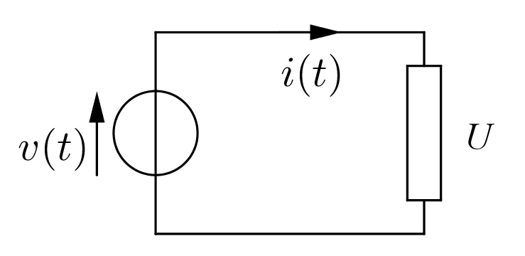
Figure 1 - Circuit with a source and a load
\(\qquad \qquad \qquad i(t)= \dfrac{\Delta q(t)}{\Delta t} \qquad \qquad i(t)= \dfrac{d\, q(t)}{d\, t}\)
the first expression being a ratio of finite changes and the second, for readers familiar with calculus, the derivative of the electric charge with respect to time.
The motion of the charges is caused by the electric field associated with the applied voltage \(\small v(t)\) and, in the case of a sinusoidal alternating emf, it consists of a harmonic oscillation of the conduction electrons as a whole in the crystal lattice.
This study is limited to steady-state currents and voltages, that is, sinusoidal currents and voltages whose characteristics, such as frequency, amplitude and phase, do not change over time. In this case we say that the electric circuit is operating under sinusoidal steady-state conditions.
1.1 - Sinusoids and complex numbers
Before going on, it is worth recalling that sinusoids can conveniently be represented by complex numbers.
Figure 2 - Vectors and complex numbers
A sinusoid \(\small y(t)\) with angular frequency \(\small \omega \) can then be represented by the complex number \(\small a+jb\) if: \(\small y(t) = \sqrt{2} \,\sqrt{a^2 + b^2} sin(\omega t + \beta)\), with \(\small \beta = arctan \left( \dfrac{b}{a}\right)\).
For a given \(\small \omega\) we therefore have the one-to-one correspondence:
\( \qquad \qquad a + j\,b\;\Longleftrightarrow\; \sqrt{2} \,\sqrt{a^2 + b^2}\, sin(\omega t + \beta) \qquad \beta = arctan \left( \dfrac{b}{a}\right)\).
and similarly for the exponential form:
\( \qquad \qquad \sqrt{a^2 + b^2}\, e^{j\,\beta}\;\Longleftrightarrow\; \sqrt{2} \,\sqrt{a^2 + b^2}\, sin(\omega t + \beta) \).
or for the polar form in Steinmetz notation:
\( \qquad \qquad \sqrt{a^2 + b^2}\, \angle \beta\;\Longleftrightarrow\; \sqrt{2} \,\sqrt{a^2 + b^2}\, sin(\omega t + \beta) \).
The factor \(\small \sqrt{2}\) is there because the magnitudes of the phasors represent RMS values rather than amplitudes.
These correspondences are the basis of the symbolic method, or phasor analysis, used to solve sinusoidal alternating current circuits.
However, as will become clear later on, not all complex numbers are interpreted as sinusoids. Some of them act as operators on the sinusoids themselves.
1.2 - Impedance
It is particularly important to be able to establish a relationship between the voltage applied by the source, \(\small v(t)\), and the current \(\small i(t)\) in the circuit. We will see that this relationship exists, but it cannot be expressed as simply as it can in direct current with Ohm's law.For now, let us write it in this form:
(1) \( \qquad \qquad \qquad \qquad v(t) = Z\, i(t) \qquad \qquad Z =\, ? \).
The quantity \(\small Z\), whose nature and mathematical structure we need to understand, is called impedance, and it can be regarded as an operator that turns one sinusoid into another: \(\small Z : i(t) \rightarrow v(t)\)

Figure 3 - The impedance operator Z turns a sinusoidal current into a sinusoidal voltage. The unit of Z is the ohm \(\small \Omega\).
Given a simple electric circuit, like the one in figure 1, with a source of sinusoidal alternating emf \(\small v(t)= V_M\,sin(\omega t)\) and an electric load U, we want to describe the current with a suitable sinusoidal function \(\small i(t)= I_M\,sin(\omega t + \theta)\), whose amplitude \(\small I_M\) and phase \(\small \theta\) must be found, and to determine the quantity \(\small Z\) that relates \(\small v(t)\) and \(\small i(t)\).
Since the impedance \(\small Z\) clearly depends on the nature and electrical characteristics of the load, we begin the analysis by studying three limiting cases:
a) a purely resistive load
b) a purely inductive load
c) a purely capacitive load
The behavior of any real load obviously shows features of all three cases, to a greater or lesser extent. Even a coil or a capacitor always has some resistance, just as the inductive and/or capacitive effects of a resistive load can never be completely eliminated. Clearly, in a coil the inductive effects will prevail, in a capacitor the capacitive ones, and so on.
Studying the limiting cases is important because it allows a simplified analysis and makes things easier to understand. The real case can then be treated as a superposition of the ideal situations studied.
2 - Purely resistive load
The load
is equivalent to an ideal resistor
(1) of resistance R
(with no inductive or capacitive effects) to which the sinusoidal
alternating voltage is applied (for simplicity, we assume the phase of the voltage is zero):(2) \( \qquad \qquad \qquad \qquad v(t) = V_M\,sin(\omega t) \).
A resistor cannot store energy. The energy it absorbs is dissipated entirely, instant by instant, as heat through the Joule effect. The device is therefore energetically passive: it simply converts all the electric energy it absorbs into heat.
Across the resistor there is a voltage drop whose instantaneous polarity is positive at the terminal where the conventional current enters.
The instantaneous positive polarities are shown by the tips of the arrows that represent the potential differences (pd).
The current \(\small i(t)\) follows exactly the waveform of the voltage \(\small v(t)\), which here coincides with the voltage drop \(\small v_R(t)\) across the resistor, according to the linear relationship:
(3) \( \qquad \qquad \qquad \qquad v_R(t) = R\,i(t) \).
that is:
(4) \( \qquad \qquad \qquad \qquad v_R(t) = R\,I_M\,sin(\omega t) \).
from which, using (2), we deduce that the amplitude of the voltage must be:
(5) \( \qquad \qquad \qquad \qquad V_M = V_{R_M} = R\, I_M \).
In terms of RMS values:
(6) \( \qquad \qquad \qquad \qquad V_R = \dfrac{V_{RM}}{\sqrt{2}} \qquad \qquad I = \dfrac{I_M}{\sqrt{2}}\).
it can be written as:
(7) \( \qquad \qquad \qquad \qquad V_R = R\, I \).
If the sinusoids are represented by the phasors \(\small \dot{V_R}\) and \(\small \dot{I}\), we find that they are in phase, that is, the angle between them is zero. The voltage \(\small \dot{V_R}\) is obtained by multiplying \(\small \dot{I}\) by the real number \(\small R\); in this case \(\small Z = R\), so:
(8) \( \qquad \qquad \qquad \qquad \dot{V_R} = R\, \dot{I} \)
A load of this kind is also called purely ohmic.
 Activity 1
 In the example
we initially set \(\small R = 4 \quad \Omega \) and an RMS voltage \(\small V = 24 \quad V\), which corresponds to
an amplitude \(\small V_M = 33.94 \quad V\).
The resistance can be changed with the
"R" slider at the bottom
left. Why an angle (0° in this case) appears in the expression
of the
 close this box
2.1 - Energy and power
We said that the resistor instantly transforms the energy \(\small w(t)\) it absorbs, converting it into heat through the Joule effect. This happens because the kinetic energy of the moving electrons is turned into vibrational energy of the atoms of the crystal lattice and of the electrons themselves.Transferring a certain amount of energy \(\small \Delta w(t)\) takes a time \(\small \Delta t\), so a power \(\small p(t) = \dfrac{\Delta w(t)}{\Delta t} =v(t)\,i(t) = R\,i^2(t) \) is involved.
This power is always positive, since it depends on the square of the current. This means that it flows in one direction only: from the source to the load.
The characteristic feature of this power is that it can be "extracted" from the electric system and, at least partly, converted into work. For example, the heat generated by the resistor can be used to heat water until it turns into steam, which, fed into a turbine connected to an alternator, makes it rotate.
Power of this kind is called active power.
To learn more about active and reactive power:
 Power in sinusoidal alternating
current
3 - Purely inductive load
A pure inductor
can be thought of as a
winding (or a solenoid) of N turns made of a
conductor completely free of resistance and capacitive effects,
characterized by a coefficient of self-induction, or
inductance, \(\small L\).The following discussion uses the concept of the derivative of a function. For a treatment that does not use calculus, see section 3.1 below.
As is well known, the self-induction coefficient \(\small L\) relates the linked magnetic flux \(\small \phi_c(t) \)(2), or self-flux, to the current that produces it:
(9) \( \qquad \qquad \qquad \qquad \phi_c(t) = L\,i(t) \)
Since this flux varies with time, a self-induced emf appears in the inductor itself, according to the well-known relationship:
(10) \( \qquad \qquad \qquad \qquad e(t) = -L\,\dfrac{d\,i(t)}{d\,t} \)
If the current \(\small i(t)\) is sinusoidal and has the form:
(11) \( \qquad \qquad \qquad \qquad i(t) =I_M\,sin(\omega t) \)
applying the rules of differentiation, from (10) we immediately get:
(12) \( \qquad e(t) = -L\,\dfrac{d\,i(t)}{d\,t} = - \omega\,L\,I_M\,cos(\omega t) = \omega\,L\,I_M\,sin \left(\omega t - \dfrac{\pi}{2}\right) \)
from which we see that \(\small e(t)\) lags the current by a quarter of a period or, as we usually say, \(\small e(t)\) is in quadrature lagging \(\small i(t)\).
The product \(\small \omega\,L\) of the angular frequency and the self-induction coefficient is denoted by \(\small X_L\), or simply \(\small X\), and is called inductive reactance:
(13) \( \qquad \qquad \qquad \qquad X_L = \omega\,L = 2\,\pi\,f\,L \)
Equation (13) also shows that \(\small X_L\) is directly proportional to the frequency.
From (12) we then have:
(14) \( \qquad \qquad \qquad \qquad e(t) = X_L\,I_M\,sin \left(\omega t - \dfrac{\pi}{2}\right) \)
So an emf \(\small e(t)\) appears across the inductor; it lags the current by a quarter of a period and has amplitude:
(15) \( \qquad \qquad \qquad \qquad E_M = X_L\,I_M \)
and RMS value:
(15') \( \qquad \qquad \qquad \qquad E = X_L\,I \qquad \qquad \qquad E= \dfrac{E_M}{\sqrt{2}}\qquad I = \dfrac{I_M}{\sqrt{2}} \)
Equations (15, 15') suggest that inductive reactance should also be measured in ohms (\(\small \Omega \)).
There is a problem, however: although they give the correct expression for the magnitudes, (15) and (15') say nothing about the phase relationships between the quantities involved. This means that equations (15, 15') do not give complete information about the behavior of the system. So how can we solve this problem?
Activity 2
To learn more about self-induction:
Self-induction under sinusoidal steady-state conditions
3.1 - Inductive reactance: a proof with rotating vectors
 It can be useful and instructive to reach the same conclusions by reasoning with
rotating vectors, without using calculus. We know (see Sinusoidal
electrical quantities) that sinusoids with the same frequency
can be represented by rotating vectors.
On the
board we see the current sinusoid \(\small i(t)\) and the corresponding rotating vector \(\small \vec{I}\)(3).
The angle \(\small \omega t\) obviously changes as time
goes by.
Let us show the situation at a generic instant \(\small t \). Now let us draw the vector in the position it occupied at an earlier instant \(\small t - \Delta t\). Between the two successive positions there is an angular distance \(\small \omega \Delta t\); this means that the current vector \(\small \vec{I}\), starting from the position \(\small \vec{I}(t - \Delta t)\), reaches \(\small \vec{I}(t)\) after \(\small \Delta t\) seconds, having swept an angle of \(\small \omega \Delta t\) radians.
In this time interval the vector \(\small \vec{I}(t)\) has changed, because, although its magnitude is the same, its direction has changed. The change must itself be a vector:
(16) \( \qquad \qquad \qquad \qquad \Delta \vec{ I} = \vec{I}(t) - \vec{I}(t - \Delta t) \)
or, if you prefer:
(17) \( \qquad \qquad \qquad \qquad \vec{I}(t) = \vec{I}(t - \Delta t) + \Delta \vec{I} \)
that is, the vector in a given position can be obtained from the vector in an earlier position by adding the change \(\small \Delta \vec{I}\).
Throughout this reasoning the parameter \(\small \Delta t\) plays a critical role, in the sense that the soundness of the argument and the accuracy of the results depend strongly on its value.
The time interval \(\small \Delta t\) must be very small, close to zero. In that case the magnitude of \(\small \Delta \vec{I}\) is practically equal to the length of the arc subtended by \(\small \vec{I}(t)\) itself and can be calculated, just like the length of the arc, as the product
(18) \( \qquad \qquad \qquad \qquad \Delta I = I_M\,\omega \Delta t \)
From (10), which here is best written in vector form (\(\small \vec{E}\) and \(\small \vec{I}\) are the rotating vectors that represent the sinusoids):
(19) \( \qquad \qquad \qquad \qquad \vec{E} = -L\, \dfrac{\Delta \vec{I}}{\Delta t} \)
we can obtain the vector \(\small \vec{E}\), which has the same direction as \(\small \Delta \vec{I}\), but points the opposite way because of the minus sign in (19). Using (18), its magnitude is:
(20) \( \qquad \qquad \qquad \qquad E = L\, \dfrac{I_M\,\omega \Delta t}{\Delta t} = \omega\,L\,I_M \)
Notice that while \(\small \Delta I\) depends on the time interval \(\small \Delta t\), \(\small E\) does not, as (20) shows.
The vector \(\small \vec{E}\) can be applied at the origin by a translation (an operation that leaves the vector unchanged, since it is moved parallel to itself without being deformed), so as to represent the sinusoid \(\small e(t)\) more easily.
Notice now that as \(\small \Delta t\) decreases, the vector \(\small \vec{E}\) tends to become perpendicular to the (rotating) vector \(\small \vec{I}\). This explains why the self-induced emf lags the current by \(\small \dfrac{\pi}{2} \).
The voltage \(\small \vec{V}\) applied by the source must be equal and opposite to \(\small \vec{E}\), because otherwise no steady current could flow.
Here too it is convenient to translate the voltage vector so that it is applied at the origin.
The applied voltage therefore leads the current in quadrature (or the current lags the applied voltage in quadrature). The board also shows the phase difference \(\small \varphi\) between them; you can check how it depends on \(\small \Delta t\), noticing that as \(\small \Delta t\) decreases it gets closer and closer to a right angle.
3.2 - Magnetic energy, power and self-induced emf
Why does the emf (10) arise, and why does it lag the current in quadrature?The current flowing through the inductor creates a magnetic field, which corresponds to an energy \(\small w\) stored in the volume of space occupied by the field:
(21) \( \qquad \qquad \qquad \qquad w(t) = \dfrac{1}{2}\,L\,i^2(t) \)
This answers both questions. The inductor is a device that stores energy in the form of a magnetic field and then releases it. Energy is stored when the emf \(\small e(t)\) opposes the current, with the inductor acting as a load. It is returned to the source when \(\small e(t)\) and the current have the same direction, and the inductor acts as a source.
The power needed to transfer the energy (21) cannot be extracted from the source-inductor system, so it cannot do work on any external system. Power with these characteristics is called reactive power.
In this exchange of energy and power, the voltage \(\small v(t)\) applied by the source must always be equal and opposite to \( \small e(t)\), so that a steady current can flow without any power being dissipated. Given, for example, (11):
(22) \( \qquad v(t) = -e(t) = L \dfrac{d\,i(t)}{d\,t}= \omega\,L\,I_M\,cos(\omega t) = \omega\,L\,I_M\,sin \left(\omega t +\dfrac{\pi}{2}\right) \)
so that:
(23) \( \qquad \qquad \qquad \qquad v(t) = X_L\,I_M\,sin \left(\omega t +\dfrac{\pi}{2}\right) \)
and therefore:
(24) \( \qquad \qquad \qquad \qquad V_M = X_L\,I_M \)
or, in terms of the RMS values \(\small V = \dfrac{V_M}{\sqrt{2}}\) and \(\small I = \dfrac{I_M}{\sqrt{2}}\):
(25) \( \qquad \qquad \qquad \qquad V = X_L\,I \)
Here too we might say that \(\small Z = X_L\) but, although true for the magnitudes, this relationship would not be entirely accurate, since relations (24) and (25), which hold for the amplitudes or their RMS values, say nothing about the relative phases of the sinusoids, for example about the fact that the sinusoid \(\small i(t)\) must lag the voltage \(\small v(t)\) by \(\small \dfrac{\pi}{2}\).
For this reason it is not enough to treat \(\small X_L\) as a simple real number.
3.3 - Inductive reactance is an imaginary number
So the
relationships between the applied voltage, the self-induced emf and the
current cannot involve only amplitudes or RMS
values, since the phase differences between the quantities
must somehow be taken into account. Let us consider once again what happens in a purely inductive circuit.
Looking at the two sinusoids we have:
\( \qquad \qquad \qquad v(t) = V_M\,sin(\omega t) \qquad \qquad i(t) = I_M\,sin \left(\omega t - \dfrac{\pi}{2}\right)\)
As we know, they correspond to the complex numbers in polar form:
\( \qquad \qquad \qquad \dot{V} = \dfrac{V_M}{\sqrt{2}}\,\angle 0° = V\,\angle 0° \qquad \quad \dot{I} = \dfrac{I_M}{\sqrt{2}}I\,\angle -90° = I\,\angle -90°\)
or in algebraic form:
\( \qquad \qquad \qquad \dot{V} = V+j\,0 \qquad \qquad \qquad \dot{I} = 0 -j\,I\)
which represent the respective phasors.
Now, to find a relationship between these quantities we could write, using the impedance operator:
\[ \dot{V} = \dot{Z}\, \dot{I}\] In fact we have already written \(\small \dot{Z}\), having realized that the impedance must itself be a complex number, since multiplying by a simple real number cannot change phase angles.
In particular, in this case, since it must produce a phase rotation of 90°, we will see that the impedance is a purely imaginary number: the complex reactance
\[ \dot{Z} = \dot{X_L} = j\,X_L\] So let us try to write the relationship we are looking for as:
\[ \dot{V} = j\,X_L\,\dot{I} \] \[ V + j\,0 = j\,X_L (0 -j\,I) \] and work out the product (note that \(\small V + j\,0 = V\) is a real number, with phase 0°):
\[ \dot{V} = j\,X_L (0 -j\,I) = -j^2 X_L\,I = -(-1) \omega\,L\,I\] which gives:
\[ V + j\,0 = \omega\,L\,I + j\,0\] which is again a real number, as indeed it had to be.
The impedance operator \(\small \dot{Z}\) applied to the phasor \(\small \dot{I}\), besides acting on its magnitude, must rotate it by \(\small \dfrac{\pi}{2}\), so that the voltage leads the current by that angle (from \(\small -\dfrac{\pi}{2}\) to \(\small 0\) in our case). So \( \dot{Z}\) must be a complex number and, in this particular case, an imaginary one. Recall in fact that (see Complex numbers, section 1.2.4, in Italian) the imaginary unit \(\small j\) can be interpreted as an operator that rotates by \(\small \dfrac{\pi}{2}\) counterclockwise. So if we represent sinusoidal quantities as phasors, which in turn are expressed by complex numbers (see Sinusoidal electrical quantities), the relationship we are looking for becomes:
(26) \( \qquad \qquad \qquad \qquad \qquad \dot{V} = j\,X_L\,\dot{I} \)
If we like, we can also write the relationship between \(\small \dot{E}\) and \(\small \dot{I}\):
(27) \( \qquad \qquad \qquad \qquad \qquad \dot{E} = -j\,X_L\,\dot{I} \)
since \(\small -j\) rotates in the opposite direction.
Finally, here are the possible forms of the inductive reactance operator:
algebraic form: \( \qquad \qquad \qquad \qquad \qquad \dot{X_L} = j\,X_L \)
exponential form: \( \qquad \qquad \qquad \qquad \dot{X_L} = X_L\,e^{\,j\,\small \dfrac{\pi}{2}} \)
polar form: \( \qquad \qquad \qquad \qquad \qquad \dot{X_L} = X_L \angle 90° \)
with magnitude: \( \qquad \qquad \qquad \qquad \qquad X_L = \omega\,L = 2\,\pi\,f\,L \quad \Omega \)
4 - Purely capacitive load
Let us now
analyze the behavior of a purely capacitive load,
which we identify with an ideal capacitor.In the dielectric of the capacitor there is an electric field produced by the charge distribution \(\small q(t)\) on the plates. This charge is related to the potential difference \(\small v(t)\) between the plates through the capacitance C, which we assume to be constant:
(28) \( \qquad \qquad \qquad \qquad \qquad d\,q(t) = C\, d\,v(t) \)
(28') \( \qquad \qquad \qquad \qquad \qquad \Delta\,q(t) = C\, \Delta\,v(t) \)
where we have used both the differential form (28) and the finite-difference form (28').
These two formulas state that any change of charge on the plates is reflected proportionally in the change of the pd between them or, conversely, that any change of pd between the plates involves a change of the charge on them. The constant of proportionality is precisely the capacitance C of the capacitor.
A change of charge, however, means that an electric current is flowing and in fact, if we divide (28) by \(\small d\,t\) or (28') by \(\small \Delta\, t\), with:
(29) \( \qquad \qquad \qquad \qquad \qquad i(t) = \dfrac{d\,q(t)}{d\,t} \)
(29') \( \qquad \qquad \qquad \qquad \qquad i(t) = \dfrac{\Delta\,q(t)}{\Delta\,t} \)
we obtain the differential equation:
(30) \( \qquad \qquad \qquad \qquad \qquad i(t) = C\, \dfrac{d\,v(t)}{d\,t} \)
or the finite-difference one:
(30') \( \qquad \qquad \qquad \qquad \qquad i(t) = C\, \dfrac{\Delta\,v(t)}{\Delta\,t} \)
If we compare (30) with (10), we can see that from a mathematical point of view the equations are formally identical (isomorphic). Only voltage and current swap roles.
Let us now derive the relationship between voltage and current using calculus:
(31) \( \qquad \qquad \qquad \qquad \qquad v(t) = V_M\, sin (\omega t) \)
from (30) we have:
(32) \( \qquad i(t) = C\,V_M\, \dfrac{d\,sin(\omega t)}{d\,t} = \omega\,C\,V_M\, cos(\omega t) = \omega\,C\,V_M\,sin \left(\omega t +\dfrac{\pi}{2} \right) \)
from which we see at once that the current sinusoid \(\small i(t)\) leads by \(\small \dfrac{\pi}{2}\) the voltage sinusoid \(\small v(t)\) across the plates of the capacitor, which coincides with the voltage at the source terminals (and also with its emf, if the source is ideal).
The amplitude of the current is:
(33) \( \qquad \qquad \qquad \qquad \qquad I_M = \omega\,C\, V_M \)
so that:
(34) \( \qquad \qquad \qquad \qquad \qquad V_M = \dfrac{1}{\omega\,C\,}\, I_M \)
a relationship that also holds for RMS values:
(35) \( \qquad \qquad \qquad \qquad \qquad V = \dfrac{1}{\omega\,C}\, I \)
We therefore set:
(36) \( \qquad \qquad \qquad \qquad \qquad X_C = \dfrac{1}{\omega\,C} = \dfrac{1}{2\,\pi\,f\,C} \)
which defines the capacitive reactance \(\small X_C\).
Notice that it is inversely proportional to the frequency.
Activity 3
4.1 - Capacitive reactance: a proof with rotating vectors
Here too it is useful to find the relationships between voltage
and current using finite-difference equations and
rotating vectors although, mathematically, this is
essentially a repetition of section 3.1, with the
appropriate changes.On the board we show the voltage sinusoid \(\small v(t)\) and the corresponding rotating vector \(\small \vec{V}\). The angle \(\small \omega t\) changes as time goes by, but let us consider the situation at a generic instant \(\small t\). Now let us draw the vector in the position it occupied at an earlier instant \(\small t - \Delta t\). Between the two successive positions there is an angular distance \(\small \omega \Delta t\), that is, the voltage vector \(\small \vec{V}\), starting from the position \(\small \vec{V}(t - \Delta t)\), reaches \(\small \vec{V}(t)\) after \(\small \Delta t\) seconds, having swept an angle \(\small \omega \Delta t\).
In this time interval the vector \(\small \vec{V}(t)\) has changed because, although its magnitude is the same, its direction has changed. The change is itself a vector:
(37) \( \qquad \qquad \qquad \qquad \qquad \vec{V}(t) - \vec{V}(t - \Delta t) = \Delta \vec{V} \)
or, if you prefer:
(38) \( \qquad \qquad \qquad \qquad \qquad \vec{V}(t) = \vec{V}(t - \Delta t) + \Delta \vec{V} \)
that is, the vector in a given position can be obtained from the vector in an earlier position by adding the change \(\small \Delta \vec{V}\).
Here too the parameter \(\small \Delta t\) plays a critical role in the accuracy and soundness of the results.
The time interval \(\small \Delta t\) must be very small, close to zero. In that case the magnitude of \(\small \Delta \vec{V}\) is practically equal to the length of the arc subtended by \(\small \Delta \vec{V}\) itself and can be calculated as the product radius x angle (in radians). In our case the role of the radius is played by the magnitude of the vector \(\small \vec{V}(t)\), while the angle is \(\small \omega \Delta t\). So:
(39) \( \qquad \qquad \qquad \qquad \qquad \Delta V = V_M\,\omega\,\Delta t \)
From (30'), which here is best written in vector form:
(40) \( \qquad \qquad \qquad \qquad \qquad \vec{I} = C\, \dfrac{\Delta\,\vec{V}}{\Delta\,t} \)
where \(\small \vec{V}\) and \(\small \vec{I}\) are the rotating vectors that represent the sinusoids, we can find the direction of the current \(\small \vec{I}\), as well as its magnitude:
(41) \( \qquad \qquad \qquad \qquad \quad I = C\, \dfrac{V_M\,\omega\,\Delta t}{\Delta\,t} = \omega\,C\,V_M \)
Notice that while \(\small \Delta V\) depends on the time interval \(\small \Delta t\), \(\small I\) does not, as (41) shows.
The vector \(\small \vec{I}\) can be applied at the origin by a translation, so as to represent the sinusoid \(\small i(t)\) more easily.
Notice now that as \(\small \Delta t\) decreases, the vector \(\small \vec{I}\) tends to become perpendicular to \(\small \vec{V}\). This explains why the current leads the voltage by \(\small \dfrac{\pi}{2}\).
The board also shows how the phase difference \(\small \varphi\) between them gets closer and closer to a right angle as \(\small \Delta t\) decreases.
4.2 - Electrostatic energy and power
When an
ideal capacitor
is connected to a source of sinusoidal alternating voltage \(\small v(t) = V_M\,sin(\omega t)\), it goes through a continuous series of charging and discharging processes.
The
charging phase
occurs when the current and the voltage applied by the source
have the same direction. In the example on the board this happens
during the first and, with reversed polarities, the third quarter of the period. In these intervals the voltage rises and the
current falls as charge builds up on the plates. The
charge distribution on the plates produces the electric field
and the corresponding potential difference \(\small v_C(t)\).
However, since the plates
are in practice the terminals of the source (the circuit is
interrupted by the dielectric), this potential difference must coincide with the voltage of the
source. Here too the phase difference between voltage and current is a sign of the system's ability to store energy.
The discharging phase occurs when the applied voltage and the current have opposite directions. This happens during the second and fourth quarters of the period. The energy previously stored in the electrostatic field is returned to the source.
The energy \(\small w\) stored in the volume of space occupied by the electrostatic field, with \(\small v_c(t) = v(t)\) as explained above, is:
(42) \( \qquad \qquad \qquad \qquad \quad w(t) = \dfrac{1}{2}\,C\, v^2(t) \)
which can be obtained, for example, by integrating the power:
(43) \( \qquad \qquad \qquad p(t) = v(t)\,i(t) = v(t)\,C\,\dfrac{d\,v(t)}{d\,t} = C\,v(t)\,\dfrac{d\,v(t)}{d\,t} \)
(44) \( \qquad \qquad \qquad w(t) = \int p(t)\,dt = C\, \int v(t)\,d\,v(t) = \dfrac{1}{2}\,C\,v^2(t) \)
up to a constant, which is zero if we assume \(\small v(0) = 0\), that is, a capacitor that is initially uncharged.
Reasoning with finite differences, we note that, by (30'), the power is given by:
(45) \( \qquad \qquad \qquad p(t) = v(t)\,i(t) = C\,v(t)\,\dfrac{\Delta\,v(t)}{\Delta\,t}\)
from which we obtain the change in energy, or the amount of work done, in the time \(\small \Delta t\):
(46) \( \qquad \qquad \qquad \Delta\,w(t)= p(t)\,\Delta t = C\,v(t)\,\Delta\,v(t)\)
Adding up the individual \(\small \Delta\,w(t)\) to get the total energy, we obtain:
(47) \( \qquad \qquad \qquad w(t) = \sum \Delta\,w(t) = C\,\sum\,v(t)\,\Delta\,v(t) = \dfrac{1}{2}\,C\,v^2(t)\)
assuming that initially v(0) = 0, that is, that the capacitor is initially uncharged.
Here too the power needed to transfer the energy (47) cannot be extracted from the system, so it cannot do work on any external system.
Power with these characteristics is called reactive power.
4.3 - Capacitive reactance is an imaginary number
We have the same problem we
had with the inductor.In a relationship between the voltage and the current of a capacitor, the capacitive reactance \(\small X_C\) cannot be a simple real number, since we must take into account the phase shift of the current, which here leads the voltage in quadrature. The voltage across the plates therefore lags the current by \(\small \dfrac {\pi}{2}\).
Using phasors we have:
(48) \( \qquad \qquad \qquad \qquad \qquad \dot{V} = -j\,X_C\,\dot{I} \)
The minus sign is there because the voltage sinusoid is obtained, apart from the change in magnitude, by rotating the current sinusoid by a lagging (clockwise) phase angle of \(\small \dfrac {\pi}{2}\).
5 - Electromotive force or voltage drop?
Whenever an energy conversion takes place in an electric load(4), a potential difference \(\small v(t)\) appears across its terminals, which in general may be a function of time. On the other hand, the energy \(\small w(t)\) is necessarily absorbed or released over a certain time, which means that electric power is involved:(49) \( \qquad \qquad \qquad p(t) = \dfrac{\Delta\,w(t)}{\Delta\,t} = v(t)\,i(t) \)
In all the situations we have analyzed, including the self-induced emf, the pd across the load always has instantaneous polarities that coincide with those of the voltage applied by the source.
Going around the circuit, this pd always appears to be opposite to that of the source. This pd is usually called a voltage drop and, as we said, it is a sign that an energy conversion is taking place.
In the particular case of the inductor, however, the pd produced by self-induction is not generated directly by the current or by the polarities of the source. It is due to a different phenomenon: the change of magnetic flux inside the inductor. For this reason it is considered to all intents and purposes an electromotive force.
6 - The series R-L circuit
An R-L circuit consists
of an ideal resistor and an ideal inductor connected in series.A load of this kind is called resistive-inductive.
The current flowing through the two devices produces the effects described above: a voltage drop \(\small v_R(t)\) across the resistor and an emf e(t) across the inductor

Figure 4 - vL(t)
is the pd
applied to the inductor
Across the inductor the source makes available a voltage \(\small v_L(t)\) that must be equal and opposite to \(\small e(t)\): \(\small v_L(t)= -e(t)\).
It might seem contradictory to represent \(\small v_L(t)\) and \(\small e(t)\) with arrows pointing the same way. However, we must bear in mind that the inductor is actually connected to the terminals A and B of an equivalent source made up of the ideal voltage source \(\small v(t)\) in series with the resistance \(\small R\). The resistance causes a voltage drop \(\small R\,i(t)\). The potential difference between terminals A and B is the voltage \(\small v_L(t)\) applied by the source to the inductor:
(50) \( \qquad \qquad \qquad v_L(t)= v(t) - R\,i(t) \)
that is:
(51) \( \qquad \qquad \qquad v_L(t)= v(t) - v_R(t) \)
From (51) it is clear that:
(52) \( \qquad \qquad \qquad v(t) = v_R(t)+ v_L(t) \)
Now, this is a sum of sinusoids, which can be represented by a sum of phasors:
(53) \( \qquad \qquad \qquad \dot{V} = \dot{V}_R + \dot {V}_L \)
On the other hand, from (8) and (26):
(54) \( \qquad \qquad \qquad \dot{V} = R\,\dot{I} + j\,X_L\,\dot{I} \)
where \(\small \dot{V_R} = R\,\dot{I}\) and \(\small \dot{V_L} = j\,X_L\,\dot{I}\) are the potential differences across the devices. Their (vector) sum is the source voltage \(\small \dot{V}\).
The three voltage phasors, with \(\small \dot{V}_L\) suitably moved (dashed vector), form the so-called voltage triangle, in which \(\small \dot{V}_R\) and \(\small \dot{V}_L\) are the legs and \(\small \dot{V}\) the hypotenuse. The angle between \(\small \dot{V}\) and \(\small \dot{V}_R\) is the phase angle \(\small \varphi\) between voltage and current. The elements of the triangle are related by the familiar trigonometric relationships:
(55) \( \qquad \qquad \qquad V_R = V\, cos(\varphi) \qquad \qquad V_L = V\, sin(\varphi)\)
Factoring out I in (54) we get:
(56) \( \qquad \qquad \qquad \qquad \dot{V} = (R + j\,X_L)\,\dot{I} \)
The expression in parentheses is the impedance of the circuit
(57) \( \qquad \qquad \qquad \qquad \dot{Z} = R + j\,X_L \)
where \(\small R\) is the real part of the impedance operator and \(\small X_L\) the imaginary part.
So:
(58) \( \qquad \qquad \qquad \qquad \dot{V} = \dot{Z}\,\dot{I} \)
From the voltage triangle we obtain the impedance triangle, whose legs are \(\small R\) and \( \small X_L\) and whose hypotenuse is \(\small Z\). Here too we have the trigonometric relationships (we omit the parentheses for simplicity):
(59) \( \qquad R = Z\,cos\,\varphi \qquad X_L = Z\,sin\,\varphi \qquad Z= \sqrt{R^2 + X^2_L} \qquad tan\,\varphi =\dfrac{X_L}{R} \)
Note that the angle φ in the impedance triangle is positive because it represents the voltage leading the current. It is a characteristic of the impedance and should not be confused with the phase angles of the vectors. The angle φ is positive for a resistive-inductive impedance and can change only if the components of the impedance itself are changed.
The role of \(\small \dot{Z}\) as a complex operator on phasors in the resistive-inductive case now becomes clearer. Acting on the vector \(\small \dot{I}\), it:
- changes its magnitude,
- changes the nature of the quantity, and therefore its unit, from amperes to volts,
- acts on the phase angle, increasing it (counterclockwise rotation) by an angle \(\small \varphi\), where: (60) \( \qquad \qquad \qquad \qquad \varphi = arctan \left(\dfrac{X_L}{R}\right) \)
You can see on the board on the left the effects of changing \(\small R\) and \(\small X_L\).
Activity 4
Inverting formula (58) we have:
(61) \( \qquad \qquad \qquad \qquad \dot{I} = \dfrac{1}{\dot{Z}}\,\dot{V} \)
or
(62) \( \qquad \qquad \qquad \qquad \dot{I} = \dot{Y}\,\dot{V} \)
which allows us to define the admittance as the reciprocal of the impedance:
(63) \( \qquad \qquad \qquad \qquad \dot{Y} = \dfrac{1}{\dot{Z}} \)
The admittance is thus the inverse operator of the impedance, \(\small \dot{Y} = \dot{Z}^{-1}\), which turns the voltage phasor into the current phasor.
As is well known, products and quotients of complex numbers are easier to work out in exponential form:
(64) \( \qquad \qquad \qquad \qquad V\,e^{j\,\alpha} = Z\,e^{j\,\varphi}\,I\,e^{j\,\beta} \)
or in Steinmetz polar form:
(65) \( \qquad \qquad \qquad \qquad V \angle \alpha = Z \angle \varphi\,I \angle \beta \)
so that \(\small \alpha = \varphi + \beta\).
For the admittance we have:
(66) \( \qquad \qquad \qquad \qquad \dot{Y} = \dfrac{1}{Z\,e^{j\,\varphi}} = \dfrac{1}{Z}\,e^{-j\,\varphi} \)
or:
(67) \( \qquad \qquad \qquad \qquad \dot{Y} = \dfrac{1}{Z}\, \angle -\varphi \)
On the other hand, \(\small \dot{Y}\) can also be written in algebraic form:
(68) \( \qquad \qquad \qquad \qquad \dot{Y} = G\,+\,j\,B \)
from which a few simple steps give the conductance \(\small G\) and the susceptance \(\small B\):
(69) \( \qquad \qquad \qquad \qquad G = \dfrac{R}{R^2+X^2_L} \qquad B = \dfrac{-X_L}{R^2+X^2_L} \)
6.1 - Power in the series R-L circuit
The resistor is characterized by the active power:(70) \( \qquad \qquad \qquad \qquad P = V_R\,I = V cos\, \varphi\,I = V\,I\,cos\,\varphi \)
and the inductor by the reactive power:
(71) \( \qquad \qquad \qquad \qquad Q = V_L\,I = V sin\, \varphi\,I = V\,I\,sin\,\varphi \)
where we have used (55).
Alternatively, recalling that in magnitude \(\small V_R = R\,I\) and \(\small V_L = X_L\,I\), we also have:
(72) \( \qquad \qquad \qquad \qquad P = V_R\,I = R\,I^2 \)
(73) \( \qquad \qquad \qquad \qquad Q = V_L\,I = X_L\,I^2 \)
7 - The series R-C circuit
An R-C circuit consists
of an ideal resistor and an ideal capacitor
connected in series. A load of this kind is called resistive-capacitive.The sum of the two pds must equal the source voltage \(\small v(t)\):
(74) \( \qquad \qquad \qquad \qquad v(t) = v_R(t) + v_C(t)\)
which translates into the relationship between phasors:
(75) \( \qquad \qquad \qquad \qquad \dot{V} = \dot{V}_R + \dot{V}_C\)
Using (48) and (8) we can write:
(76) \( \qquad \qquad \qquad \qquad \dot{V} = R\,\dot{I} - j\,X_C\,\dot{I}\)
where \(\small \dot{V}_R = R\,\dot{I}\) and \(\small \dot{V}_C = - j\,X_C\,\dot{I}\) are the potential differences across the devices. Their (vector) sum is the source voltage \(\small \dot{V}\).
The three voltage phasors, with \(\small \dot{V}_C\) suitably moved (dashed vector), form the so-called voltage triangle, in which \(\small \dot{V}_R\) and \(\small \dot{V}_C\) are the legs and \(\small \dot{V}\) the hypotenuse. The angle between \(\small \dot{V}\) and \(\small \dot{V}_R\) is the phase angle \(\small \varphi\) between voltage and current. The elements of the triangle are related by the familiar trigonometric relationships:
(77) \( \qquad \qquad \qquad V_R = V\, cos(\varphi) \qquad \qquad V_C = V\, sin(\varphi)\)
Factoring out \(\small \dot{I}\) in (76):
(78) \( \qquad \qquad \qquad \qquad \dot{V} = (R - j\,X_C)\,\dot{I}\)
while the impedance is:
(79) \( \qquad \qquad \qquad \qquad \dot{Z} = R - j\,X_C\)
Note that because the imaginary part of \(\small \dot{Z}\) is negative, the angle \(\small \varphi\) is negative as well:
(80) \( \qquad \qquad \qquad \qquad \varphi = arctan\left( \dfrac{-X_C}{R} \right)\)
In the resistive-capacitive case the operator \(\small \dot{Z}\), acting on the vector \(\small \dot{I}\):
- changes its magnitude,
- changes the nature of the quantity, and therefore its unit, from amperes to volts,
- acts on the phase angle, decreasing it (clockwise rotation) by an angle \(\small \varphi = arctan\left( \dfrac{-X_C}{R} \right)\)
Activity 5
For the admittance we have:
(81) \( \qquad \qquad \qquad \qquad \dot{Y} = \dfrac{1}{Z\,e^{-j\,\varphi}} = \dfrac{1}{Z}\,e^{j\,\varphi} \)
or:
(82) \( \qquad \qquad \qquad \qquad \dot{Y} = \dfrac{1}{Z}\, \angle \varphi \)
On the other hand, \(\small \dot{Y}\) can also be written in algebraic form:
(83) \( \qquad \qquad \qquad \qquad \dot{Y} = G\,+\,j\,B \)
from which a few simple steps give the conductance \(\small G\) and the susceptance \(\small B\):
(84) \( \qquad \qquad \qquad \qquad G = \dfrac{R}{R^2+X^2_C} \qquad B = \dfrac{X_C}{R^2+X^2_C} \)
Notice here too the difference in the sign of the susceptance compared with the resistive-inductive case.
7.1 - Power in the series R-C circuit
The resistor is characterized by the active power:(85) \( \qquad \qquad \qquad \qquad P = V_R\,I = V cos\, \varphi\,I = V\,I\,cos\,\varphi \)
and the capacitor by the reactive power:
(86) \( \qquad \qquad \qquad \qquad Q = - V_C\,I = - V sin\, \varphi\,I = - V\,I\,sin\,\varphi \)
where we have used (77).
Alternatively, recalling that in magnitude \(\small V_R = R\,I\) and \(\small V_C = X_C\,I\), we also have:
(87) \( \qquad \qquad \qquad \qquad P = V_R\,I = R\,I^2 \)
(88) \( \qquad \qquad \qquad \qquad Q = -V_C\,I = - X_C\,I^2 \)
As you can see, given the relationships between the quantities involved, the capacitive reactive power is negative.
This last statement is easier to understand if we take the current as the reference, both in the R-C and in the R-L case (change the angle α until the current vector lies on the real axis and so has zero phase): \(\small V_L\) and \(\small V_C\) are opposite, \(\small V_L\) is positive and \(\small V_C\) is negative. Inductive reactive power is positive, capacitive reactive power is negative.
8 - The series R-L-C circuit
In the R-L-C circuit all
three basic components are connected in series.Thanks to what we have learned so far, we can write the impedance directly:
(89) \( \qquad \qquad \qquad \qquad \dot{Z} = R + j\,X_L - j\,X_C = R + j\,(X_L - X_C)\)
Depending on the values of the reactances, the current can
- lead
- be in phase with
- lag
So overall the circuit can behave as:
- capacitive
- resistive
- inductive
Of particular interest, because of its implications for the efficient use of electric power(5), is the case in which \(\small X_L = X_C\), which, as (89) shows, makes the imaginary part of the impedance zero. The load then appears to be resistive, even though an inductor and a capacitor are present.
Activity 6
The potential differences across the devices add up (as vectors) to the source voltage V.
8.1 - Energy exchanges in the series R-L-C circuit
In the previous analyses we described the energy behavior of the individual devices. To sum up:- The resistor converts energy into heat without storing it. The power is active: it flows only from the source to the load. The power leaves the system (as heat, in this case).
- The inductor stores energy in the form of a magnetic field during certain time intervals. The energy is returned to the source during other intervals. There is no dissipation. The power flows in both directions and is reactive. It cannot leave the system. It cannot do work outside the system.
- The capacitor stores energy in the form of an electric field during certain time intervals. The energy is returned to the source during other intervals. There is no dissipation. The power flows in both directions and is reactive. It cannot leave the system. It cannot do work outside the system.
You can understand this by looking at the arrangement of the voltage and current vectors on the devices, whose relationship with energy and power we discussed earlier.
In other words, the inductor and the capacitor behave in complementary ways. So all or part of the reactive energy and power can be exchanged between them, involving the source only partly or not at all (when XL = XC).
Activity 7
9 - Voltage resonance
It is very interesting to analyze how the inductive and
capacitive reactances behave as the frequency changes.
From figure 5, and bearing in mind the now familiar expressions for inductive and capacitive reactance, which we repeat here:
\( \qquad \qquad \qquad \qquad \qquad X_L = 2\,\pi\,L\,f \)
\( \qquad \qquad \qquad \qquad \qquad X_C = \dfrac{1}{2\,\pi\,C\,f} \)
we can see that inductive reactance grows linearly with frequency, while capacitive reactance follows a hyperbola, being inversely proportional to frequency.
We can also notice that at \(\small f = 0\) Hz, which corresponds to direct current, the ideal inductor behaves like a short circuit, \( \small X_L = 0\), while the ideal capacitor is a break in the circuit, that is, an open circuit, \(\small X_C = \infty\).
A circuit with an inductor in series tends to cut high frequencies, the more so the higher the inductance (low-pass filter). A capacitor in series, instead, cuts low frequencies, the more so the smaller the capacitance C (high-pass filter).
Figure 5 - Inductive and capacitive reactance as a function of frequency
There is a value of the frequency, called the resonant frequency \(\small f_R\), at which the two curves intersect. At this frequency the two reactances are equal, \(\small X_L = X_C\), and the impedance \(\small Z = R + j\,( X_L - X_C)\) takes its minimum value, equal to \(\small R\). As a result the current reaches a maximum.
We then say that the system is in resonance. In this case we speak of series resonance or voltage resonance.
At resonance the current is limited by the resistance alone, and the applied voltage and the current are exactly in phase.
Activity 8: resonance
From an energy point of view, we can say that resonance is characterized by a balanced exchange of power between the reactive components. The two powers are equal and opposite in sign, which means that while one component absorbs reactive energy (power), the other releases exactly the amount needed. As far as reactive power is concerned, the system becomes independent of the source.
There is, of course, a formula for finding \(\small f_R\) when \(\small L\) and \(\small C\) are known.
If \(\small X_L = X_C\), we have \(\small 2\,\pi\,L\,f= \dfrac{1}{2\,\pi\,C\,f}\) and therefore \(\small (2\,\pi)^2\,L\,C\,f^2 = 1\), which gives the resonant frequency:
(90) \( \qquad \qquad \qquad \qquad f_R = \dfrac{1}{2\,\pi\,\sqrt{L\,C}}\)
Voltage resonance is potentially dangerous, because even with a modest supply voltage high currents can flow, which across the reactive components (inductor and capacitor) produce very high potential differences. This happens because when the reactances are equal the imaginary part of the impedance vanishes, so that only the resistance limits the current. If \(\small R\) is very small, the current is correspondingly large. In the limit, for \(\small R = 0\), we would have a short circuit, with current and voltages tending to infinitely large values.
Activity 9
In fact the impedance reaches its minimum value at the resonant frequency, where the current reaches its maximum.
Not only the impedance depends on frequency, but also its characteristic angle \(\small \varphi\).
Figure 6 - Impedance and phase angle as a function of frequency
The angle \(\small \varphi\) of the impedance rotates as the frequency changes, as figure 6 shows. It passes through zero exactly at the resonant frequency. Above the resonant frequency the angle \(\small \varphi\) is positive and the circuit is resistive-inductive (or simply inductive if R=0); below the resonant frequency \(\small \varphi\) is negative and the circuit is resistive-capacitive. At the resonant frequency \(\small \varphi = 0\) and the circuit behaves as a purely resistive one. We can also study the frequency behavior in the R-L case, where we can clearly see how the current is attenuated at high frequencies, and in the R-C case, where the attenuation occurs at low frequencies.
Activity 10
Next module: Previous module:
- Alternating Current 1: sinusoidal electrical quantities, generation, phasors and the symbolic method
Rev. October 2026; English version October 2026
Books by the author
The author’s books
(1) The device, the resistor, is very often confused with its electrical property, the resistance. The same happens with inductor (the device) and inductance (the property). With the capacitor, instead, capacitor correctly refers to the device and capacitance to the electrical property

(2) A solenoid with \(\small N \) turns, cross-section \(\small S\) and length \(\small l\) carrying a current \(\small I\) produces a magnetic flux \(\small \Phi = \mu\,\dfrac{S}{l}\,N\,I\ = \dfrac{N\,I}{\mathcal{R}} \), where \(\small \mathcal{R}\) is the magnetic reluctance. The linked flux is \(\small N\) times the flux \(\small \Phi\), since it links the same \(\small N\) turns: \(\small \Phi_C = \dfrac{N^2}{\mathcal{R}}\,I = L\,I \)
(3) As an exception to the notation used in these lessons, here we also write \(\small \vec{I}(t)\) and \(\small \vec{I}(t - \Delta t)\) to express how the position of the rotating vector depends on time.
(4) An energy conversion in an electric circuit involves a motion of charges, and therefore a current \(\small i(t)\), between two points A and B of the circuit with a potential difference \(\small V_{AB}\) between them. A has a positive instantaneous polarity if, with respect to a common potential reference, \(\small V_A(t) > V_B(t)\). Otherwise A has zero instantaneous polarity if \(\small V_A(t)= V_B(t)\), or negative polarity if \(\small V_A(t) < V_B(t)\).
(5) The technique of bringing the current into phase with the voltage is called power factor correction. It allows electrical installations to make better use of electric energy. In practice a capacitor is connected not in series but in parallel with a resistive-inductive load, because the voltage across the load must not change, so as not to alter the way it operates.