Electrical technology › Power factor correction

Power factor correction in electrical installations

Rifasamento degli impianti elettrici

1 - Reactive power

Almost all industrial electrical loads behave like a resistive-inductive impedance, so the current lags the voltage by an angle \(\small \varphi_u\)⁽¹⁾. This phase shift means that there is an exchange of reactive power between generator and load. Electric motors, for example, work through the interaction of a magnetic field with the currents flowing in their circuits. Building up the magnetic field requires the energy carried by reactive power, inductive in this case. As is well known, reactive power cannot be used to do work outside the electrical system, but it still has to be produced by the generators and made available to the devices that need it. It is continuously exchanged between generators and loads and occupies the transmission lines with the corresponding current, also called reactive current.

Activity 1

2 - Active current and reactive current

The current drawn by the load can be split into two components:
the active current, in phase with the voltage, given by:

\[I_a = I_u\,cos\,\varphi_u \]
and the reactive current already mentioned, in quadrature with the voltage:

\[I_r = I_u\,sin\,\varphi_u \]

Of course, for a given supply voltage V, the active component is proportional to the active power:

\[P_u = V\,I_u\,cos\,\varphi_u = V\,I_a \]

while the reactive component is proportional to the reactive power:

\[Q_u = V\,I_u\,sin\,\varphi_u = V\,I_r \]
The supply network and the generators must deliver to the load both the active power, which will be used to do work, and the reactive power it needs.
However, we know that inductors and capacitors behave in complementary ways as far as reactive power is concerned: supplied by the same sinusoidal AC voltage, the capacitor delivers reactive power when the inductor absorbs it, and vice versa.

3 - Power factor correction

This suggests that the exchange of reactive energy, which normally takes place between load and generator, could instead take place between a resistive-inductive load and a capacitor connected in parallel with the load itself.
The parallel connection is of course meant to leave the voltage across the load (simulated by the R-L impedance) unchanged, and therefore the way the load itself works.
If we connect the capacitor we immediately see that the phase angle is reduced and at the same time the magnitude of the current decreases.
Looking more closely, we also notice that the current drawn by the load \(I_u\) has not changed.
The current in the capacitive branch, leading the voltage by 90°, added to the current \(I_u\), gives the total line current \(I_T\).
The phase angle φ_u has not changed either, which confirms that the load works exactly as it did before the capacitor was connected, drawing the same current, the same active power and the same reactive power.
The reactive power carried by the line has decreased instead, because part of the energy exchange now takes place directly between inductor and capacitor. In fact the reactive component of the total current has decreased.
The active component of the current stays constant, which confirms that the active power drawn does not change. On the other hand the capacitor only absorbs reactive power and so cannot change the situation in that respect.
If we also draw the reactive component \(\small I_{ur}\) of the current drawn by the load, we can write a few important relations. For example:

\[I_a = I_T\,cos\,\varphi = I_u\,cos\,\varphi_u\]
which states that the active components of the total current \(I_T\) and of the load current \(I_u\) are equal.
The reactive component of the total current can be found from the active component:

\[I_r = I_T\,sin\,\varphi = I_a\,tan\,\varphi\]

and the same holds for the reactive component of the load current \(I_{ur}\):

\[I_{ur} = I_u\,sin\,\varphi = I_a\,tan\,\varphi_u\]

From the phasor diagram we see that the capacitor current can be seen as the difference between the two reactive components:

\[I_c = I_{ur} - I_r\]
Using the previous formulas:

\[I_c = I_a\,(tan\,\varphi_u - tan\,\varphi)\]
Multiplying both sides of this relation by V we get:

\[V\,I_c = V\,I_a\,(tan\,\varphi_u - tan\,\varphi)\]
and therefore:

\[V\,I_c = V\,I_u\,cos\,\varphi_u\,(tan\,\varphi_u - tan\,\varphi)\]
Since \(V\,I_c = Q_c \) is the reactive power absorbed by the capacitor, while \(V\,I_u\,cos\,\varphi_u \) is clearly the active power absorbed by the load:

\[Q_c = P_u\,(tan\,\varphi_u - tan\,\varphi)\]
This is also called the correcting reactive power.
Since:

\[Q_c = \frac{V^2}{X_c} = \frac{V^2}{\frac{1}{\omega C}} = \omega\,C\,V^2\]
we can find the correcting capacitance:

\[C = \frac{P_u}{\omega V^2}\,(tan\,\varphi_u - tan\,\varphi)\]

Activity 2: Problem

A load draws, at 230 V, 50 Hz, an active power of 5 kW and an inductive reactive power of 8 kvar, and is supplied by a line with impedance 0.2 + j 0.3 Ω. We want to correct the load to a power factor of 0.9 while keeping the voltage at the receiving end of the line at 230 V. Find the capacitance to connect in parallel, the load current after correction, the total line current and the voltage drop on the line as a percentage of the receiving-end voltage.

Let us find the apparent power:

\[S = \sqrt{P^2 + Q^2} = \sqrt{5^2 + 8^2} = 9.43 \;\;kVA\]

from which we get the current drawn:

\[I = \frac{S}{V} = \frac{9430}{230} = 41\;\;A \]
and the power factor:

\[cos\,\varphi_u = \frac{P}{S} = \frac{5}{9.43} = 0.530\]
\[\varphi_u = arccos\,0.530 = 58° \]
Taking the phase of the voltage as zero:

\[V = 230\, \angle 0°\;\;V \]
the current has phase -58° and, in polar form:

\[I = 41\, \angle -58°\;\;A \]
The power dissipated on the supply line is:

\[P_l = R_l\,I^2 = 0.2 \cdot 41^2 = 336\;\;W\]

The voltage at the sending end of the line can be found with the approximate formula for the voltage drop used in industrial practice:

\[V_0 = V + I ( R_l\, cos\, \varphi_u + X_l\,sin\,\varphi_u) \]
so:

\[V_0 = 230 + 41\,( 0.2 \cdot 0.530 + 0.3 \cdot 0.848) = 245\;\;V \]
We can now find the correcting capacitance for a power factor of 0.9, which corresponds to:

\[\varphi = arccos\,0.9 = 25.8° \qquad tan\,\varphi = 0.484\]
and therefore:

\[C = \frac{P}{\omega V^2}(tan\, \varphi_u - tan\, \varphi)\]

that is:
\[C = \frac{5000}{314 \cdot 230^2}(1.6 - 0.484) = 336\;\;\mu F\]

after correction the line current is:
\[I = \frac{P}{V\,cos\, \varphi} = \frac{5000}{230 \cdot 0.9} = 24\;\;A\]
In polar form:

\[I = 24\, \angle -25.8°\;\;A \]
Line losses equal to:

\[P_l = R_l\,I^2 = 0.2 \cdot 24^2 = 115\;\;W\]

and a sending-end voltage of:

\[V_0 = 230 + 24\,( 0.2 \cdot 0.9 + 0.3 \cdot 0.436) = 237.5\;\;V \]

Check the current and power factor values on the board on the left. To do this you will have to set the circuit parameters appropriately, with a few calculations. Follow the steps below and answer the questions (use a decimal point). If the answer is correct, the right value will be set:

In theory the load could be fully corrected, bringing the total current in phase with the voltage. In that case, since \(\varphi = 0\) and \(tan\,\varphi = 0\), we would have:

\[C = \frac{P\,tan\,\varphi_u}{\omega\,V^2} = \frac{Q_u}{\omega\, V^2}\]
but this is not normally the goal, because an "overcorrection", which could occur when operating conditions change, must be strictly avoided, as it would make the load capacitive overall. Capacitive loads are undesirable because of the overvoltages they can cause at the receiving end of the supply line (Ferranti effect, fig. 1).

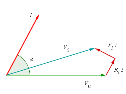
Fig. 1 - The Ferranti effect. With strongly capacitive loads the receiving-end voltage \(\small V_u\) of the line can exceed the sending-end voltage \(\small V_0\).

4 - Power triangle

The effect of power factor correction is very clear if we look at the power triangle. When we connect the capacitor the active power stays the same while the total reactive and apparent power decrease, even though the reactive power absorbed by the load does not change.
As already said, capacitive reactive power must not be fed into the network, so as a precaution the power factor is corrected to a value below unity.
In Italy the electricity distributor uses 0.9 as the reference value.
Installations with a lower power factor are penalized with a higher energy price. If the power factor is 0.7 or lower, correction is mandatory.

5 - Ratings of the capacitor bank

A capacitor bank of capacitance C delivers its rated reactive power when it is supplied at its rated voltage:

\[Q_{Cn} = \frac{V_n^2}{X_C} = \omega\,C\,V_n^2 \]
which clearly depends on the square of the voltage.
If the bank is used at a voltage different from its rated voltage, at the same frequency, the correcting power is:

\[ Q_C = \omega\, C\, V^2 = Q_{Cn}\,\frac{V^2}{V_n^2}\]

Then, since:

\[I_C = \frac{V}{X_C} = \omega\,C\,V\]
the rated current is:

\[I_{Cn} = \omega\,C\,V_n \]
and therefore:

\[I_C = I_{Cn}\, \frac{V}{V_n}\]

6 - Three-phase power factor correction

In a three-phase system, the correcting capacitance also depends on how the capacitors are connected.
With capacitor banks connected in star (wye), if V is the line-to-line voltage and E the phase voltage, we have:

\[C_Y = \frac{P}{3\,\omega\, E^2}\,(tan\,\varphi_u - tan\,\varphi)\]

and since \(\small E = \dfrac{V}{\sqrt{3}}\), substituting into the previous formula:

\[C_Y = \frac{P}{3\,\omega\, \left(\frac{V}{\sqrt{3}} \right)^2}\,(tan\,\varphi_u - tan\,\varphi) = \frac{P}{\omega\, V^2}\,(tan\,\varphi_u - tan\,\varphi)\]

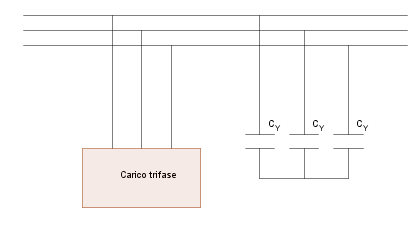
Fig. 2 - Three-phase power factor correction with star-connected capacitors

In the delta connection, since V is also the phase voltage:

\[C_D = \frac{P}{3\,\omega\, V^2}\,(tan\,\varphi_u - tan\,\varphi)\]

The conclusion is that with this connection we get the same effect using capacitors with one third of the capacitance needed with the star connection:

\[C_D = \frac{C_Y}{3}\]
For this reason, at low voltage, capacitor banks are always connected in delta.
At medium-high voltages the star connection may be preferable for insulation reasons, since the capacitors can then be rated for a voltage \(\sqrt{3}\) times lower.

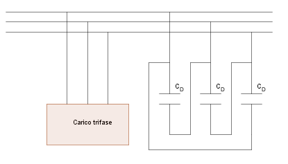
Three-phase correction, delta connection

Fig. 3 - Three-phase power factor correction with delta connection

7 - Benefits of power factor correction and regulations

To sum up, the benefits of correct power factor correction are:

lower line current under the same operating conditions of the loads; it is therefore possible to reduce the cross-section of the conductors or to supply more loads with the same line
lower line losses, which are proportional to the square of the current
lower voltage drops on the line

Rules in Italy for installations with a contracted power above 16.5 kW:

the monthly average power factor cannot be below 0.7
the minimum instantaneous power factor at maximum load during peak periods is 0.9
with 0.7 < cos φ < 0.95 the energy in time bands F1 and F2 is subject to a surcharge
feeding (capacitive) reactive power into the network is strictly forbidden (overcorrection)

For the regulations see the website of the Italian Regulatory Authority for Energy, Networks and Environment (ARERA), in particular resolution 180/2013/R/eel (in Italian).

8 - Related topics and further reading

Electric power in sinusoidal AC circuits
The author’s books
AC 1: sinusoidal electrical quantities
AC 2: impedance, reactance, series RLC, voltage resonance (in Italian)
AC 3: admittance, parallel RLC, current resonance (in Italian)
Complex numbers 1: definitions and basic operations (in Italian)
Complex numbers 2: Euler's formula, complex powers and logarithms (in Italian)

⁽¹⁾ The subscript 'u' refers to the quantities of the load, here simulated by a resistive-inductive impedance. Any device that draws electric power is called a load (electrical load).